Introduction

In the last few decades, there has been a "Probability Revolution" within the sciences, changing the way research is done, and opening up many opportunities for new interpretation and extrapolation of data. In Computer Science, probability is an essential component in algorithms for search results, matching, machine learning and artificial intelligence rely on probability. In this section we will look at some key aspects of probability for Computer Science.

Probability Event

Within an event, the set of all possible outcomes is called the Sample Space, which is denoted as set S.

For example, if we toss a coin, we have: S = {heads, tails}

If we roll a die, we have: S = {1, 2, 3, 4, 5, 6}

If we select a suite of cards, we have: S = {hearts, diamonds, clubs, spades}

A more complex example might be the flipping of two coins, where we have: S = {(heads, heads), (heads, tails), (tails, heads), (tails, tails)}

With this in view, we can define an event as a collection of outcomes of interest. What does this mean? Well, for example, if we were to roll two dice and were interested in getting a double, the event A would be defined as:

A = {(1,1), (2,2), (3,3), (4,4), (5,5), (6,6)}

A similar example would be an event B, where the sum of the two dice is less than 4. We would then define B as:

B = {(1,1), (1,2), (2, 1)}

Mutually Exclusive

If two events have no elements in common, then we say that they are mutually exclusive. For example, if B is the event where the sum of the two dice is less than 4, and C is the event where the sum of the two dice equals 5, we have:

B = {(1,1), (1,2), (2, 1)}
C = {(1,4), (2, 3), (3, 2), (4, 1)}

Notice than there are no elements in common between B and C. Thus, B and C are mutually exclusive.

Combining Events

Event Operators:

• ~ : Not
• ∩ : And
• U : Or

As you might have already noticed, Events are represented mathematically as Sets (Click here to review Set Theory). As such, the same operations possible on set may be applied to probability events. Thus, the NOT, AND and OR operations follow the behavior of Sets.

Rules

The probability of even A occurring is denoted as: P[A]

The primary rules governing the nature of P[A] are as follows:

1. 0 ≤ P[A] ≤ 1
2. P[S] = 1
3. For mutually exclusive events A and B, P[A U B] = P[A] + P[B]

To elaborate further, the first rule (1) indicates that the probability of an event occurring is expressed as a real number between 0 and 1. For example, if there is a 50%, the real number value will be 0.5 .

The second rule, P[S] = 1, explicitly defines the probability of the entire sample space of events as equating to 100% probability of occurring. Lastly, the third rule states that the probability of the union of two mutually exclusive events is equal to the sum of the probabilities of the events.

Thus, if we have a sample space of coin tosses:

S = {heads, tails}

We would have the following:

P[heads] = 0.5
P[tails] = 0.5
P[S] = 1
P[heads U tails] = P[heads] + P[tails] = 0.5 + 0.5 = 1

Conditional Probability

Sometimes the probability of an event occurring is dependent on another event occurring. For example, if you were interested in the probability that it is a Friday and a student is absent, you would need to take both factors (probability of being absent, and the probability of it being a Friday) into consideration.

To solve such a situation, we use conditional probability. The formula for conditional probability is as follows:

P(B|A) = P(A ∩ B) / P(A)

This is read as "The probability of B given A is equal to the Probability of A and B over the Probability of A.

In our example of the "probability that it is a Friday and a student is absent", knowing that the probability of a student being absent is 0.03 and that the probability of it being a Friday is 0.2 (there are five days in a school week), therefore, we would calculate the conditional probability as follows:

let P(A) be the probability of a child being absent.
let P(F) be the probability of it being a Friday.
given P(A) = 0.03
given P(F) = 0.2
P(A|F) = P(A ∩ F) / P(F)
       = 0.03 / 0.2
       = 0.15

So we have found that there is a 15% probability that it is Friday and a child is absent.

Bayes Theorem

A more common scenario when dealing with conditional probability is where the probability of an event is "updated" by supporting evidence of the occurrence of that event. In such a situation we would make use of Bayes Theorem.

Wikipedia has a very nice introductory example to illustrate this concept, which goes as follows:

"Suppose a man told you he had a nice conversation with someone on the train. Not knowing anything about this conversation, the probability that he was speaking to a woman is 50% (assuming the train had an equal number of men and women and the speaker was as likely to strike up a conversation with a man as with a woman). Now suppose he also told you that his conversational partner had long hair. It is now more likely he was speaking to a woman, since women are more likely to have long hair than men. Bayes' theorem can be used to calculate the probability that the person was a woman.

To see how this is done, let W represent the event that the conversation was held with a woman, and L denote the event that the conversation was held with a long-haired person. It can be assumed that women constitute half the population for this example. So, not knowing anything else, the probability that W occurs is P(W) = 0.5.

Suppose it is also known that 75% of women have long hair, which we denote as P(L |W) = 0.75 (read: the probability of event L given event W is 0.75, meaning that the probability of a person having long hair (event "L"), given that we already know that the person is a woman ("event W") is 75%). Likewise, suppose it is known that 15% of men have long hair, or P(L |M) = 0.15, where M is the complementary event of W, i.e., the event that the conversation was held with a man (assuming that every human is either a man or a woman).

Our goal is to calculate the probability that the conversation was held with a woman, given the fact that the person had long hair, or, in our notation, P(W |L). Using the formula for Bayes' theorem, we have:

where we have used the law of total probability to expand P(L). The numeric answer can be obtained by substituting the above values into this formula (the algebraic multiplication is annotated using " · ", the centered dot). This yields

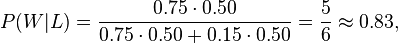
i.e., the probability that the conversation was held with a woman, given that the person had long hair, is about 83%."

Mathematical Expectation

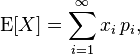
Sometimes we are interested, not in the occurrence of a single event, but of the potential cumulative effect of events over time. For this, we use mathematical expectation which can be defined as a "weighted average of all possible numbers".

To calculate this, we calculate the sum of all values multiplied by their probabilities.

As a simple example, suppose we would like to know the mathematical expectation of 10 coin tosses, where heads is 0 and tails is 1. The summation of the ten events weighted by their proabilities would be:

E[X] = 0.5(1) + 0.5(1) + 0.5(1) + 0.5(1) + 0.5(1) + 0.5(1) + 0.5(1) + 0.5(1) + 0.5(1) + 0.5(1)
E[X] = 5

Probability Distributions

Wikipedia defines a Probability Distribution as follows:

> a probability distribution assigns a probability to each measurable subset of the possible outcomes of a random experiment, survey, or procedure of statistical inference.

This, in essence, means that for each possible event in the sample space, a probability value is assigned. When graphed, this provides us with a more intuitive understanding of how the probability behaves across the universe of events. For example, if we graphed the probability distribution of the height of adults, we would not expect a uniform probability across every possible value (for example, it is not equally probable that an adult is 5 inches tall than 5 foot tall). Here is an example of a height distribution for men and women:

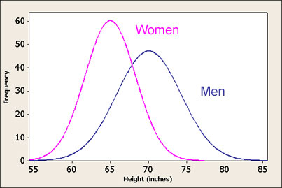
In the above graph, the sample event space is the values along the bottom x-axis, and the relative probability for each x-value becomes the corresponding y-value which is then plotted to produce the curve(s) which is then referred to as the probability distribution.

Discrete Probability Distributions

Discrete Uniform Distribution

The Discrete Uniform Distribution, is the a probability distribution where, for all x-values, the y-value is constant.

Binomial Distributions

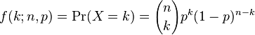
We use the Binomial Distribution when we have a series of trials, where the outcome of each trial is either Success or Failure (true or false). If we assume that the probability for a trial being successful is a constant value p, then the probability of the failure would logically be, therefore, 1 - p.

The probability of X successes in n trials is calculated as:

From this, we deduct the following two properties:

1. E[X] = np (Mathematical Expectancy)
2. var(X) = np(1 - p) (Variance)

As an example, suppose that the probability that a person will survive a serious blood disease is 0.4. If 15 people have the disease, we can say that the number of survivors, X, has a Binomial B(15, 0.4) distribution. Using the above equation, we would calculate probability by plugging in the values:

n = 15
p = 0.4

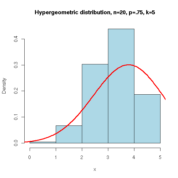
Hypergeometric Distributions

A relative of the Binomial distribution is the hypergeometric distribution. This probability distribution describes the probability of k successes in n draws without replacement from a finite population of size N containing exactly K successes. The main point of difference between this distribution and the binomial distribution is that the binomial distribution allows for replacement, whereas the hypergeometric distribution does not.

We calculate probability in the hypergeometric distribution as follows:

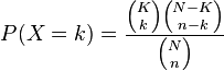
Let's examine an example from Wikipedia:

In Hold'em Poker players make the best hand they can combining the two cards in their hand with the 5 cards (community cards) eventually turned up on the table. The deck has 52 and there are 13 of each suit. For this example assume a player has 2 clubs in the hand and there are 3 cards showing on the table, 2 of which are also clubs. The player would like to know the probability of one of the next 2 cards to be shown being a club to complete his flush.

There are 4 clubs showing so there are 9 still unseen. There are 5 cards showing (2 in the hand and 3 on the table) so there are 52-5=47 still unseen.

The probability that one of the next two cards turned is a club can be calculated using hypergeometric with k=1, n=2, K=9 and N=47. (about 31.6%)

The probability that both of the next two cards turned are clubs can be calculated using hypergeometric with k=2, n=2, K=9 and N=47. (about 3.3%)

The probability that neither of the next two cards turned are clubs can be calculated using hypergeometric with k=0, n=2, K=9 and N=47. (about 65.0%)

Poisson Distributions

The Poisson Distribution describes the probability of a given number of events occurring within a fixed interval of time (and/or space) if these events occur with a known average rate and independently of the time since the last event. In other words, it predicts the probability spread around a known average rate of occurrence.

A discrete random variable X is said to have a Poisson distribution with parameter λ > 0, if, for k =0,1,2,...,n, the probability mass function of X is given by:

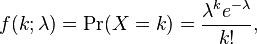
where

• e is Euler's number (e = 2.71828...)
• k! is the factorial of k.
• The positive real number λ is equal to the expected value of X and also to its variance

Here is an example to illustrate the Poisson distribution as a graph:

For example, if we knew that the average number of oil tankers arriving at a port per day is 10, and we know that the port is capable of accommodating 15 tankers per day as a maximum. What is the probability that on a particular day the port will be unable to support the number of oil tankers?

In this case, the variable X is

Poisson λ = 10

thus, we calculate the probability as follows:

Exercises

Continue to the next section