Objectives

In this session you will learn the following:

1. Plotting 2 dimensional line graphs
2. Annotating graphs with grids, axis labels, graph titles
3. Exporting graphs for inclusion in documents
4. Plotting 3 dimensional surface graphs
5. Plotting multiple graphs on one page (subplot())

Functions for Plotting

In this session, we will learn the following functions:

plot(), plot2d(), xgrid(), xtitle(), legend(), plot3d(), linspace()

Plotting Basics

Scilab is a data plotter, that is, it plots graphs from the data you input. This is in contrast to function plotting programs (such as gnuplot) which plot graphs of functions without the user having to first explicitly generate the data required to plot the graph. Function plotting programs will decide the range of the values of independent variable and its data interval, generate the data on the fly and plot the graph.

Let us plot a graph of sin(x) and cos(x) over the range x = 0 to 2 pi. We will first create vector x, containing the values of the independent variable x. Then we will create the matrix y, containing the same number of rows as x, with values of sin(x) in its first column and values of cos(x) in its second column.

-->x = [0:%pi/16:2*%pi]';
-->y = [sin(x), cos(x)];
-->plot(x, y); xgrid(1); xtitle('Harmonic Functions', 'x', 'sin(x) and cos(x)');

This must result in the following graph being plotted:

Let  me explain how this was achieved:

1. Using the plot() function, we told Scilab to look for values of x in the first variable (namely x) and look for values of y in the second variable (namely y). The number of rows in x and y must be the same. Since y contains two columns, Scilab understands that it must plot two lines in the graph, one each for each column of values.
2. Using xgrid() function, we told Scilab to plot grids parallel to the x- and y-axes in black color (argument 1 to the function xgrid()).
3. Using the xtitle() function, we defined the title of the graph (first argument), title for the x-axis (second argument) and title for the y-axis (third argument).

In the same way, we could define a legend with the legend() function as follows:

-->plot(x, y); xgrid(1); xtitle('Harmonic Functions', 'x', 'sin(x), cos(x)'); legend(['sin(x)', 'cos(x)'], 3)

First argument to legend() is an array of strings containing the legend text and the second argument specifies the position. Use the online help to learn more about the legend() function.

Interactive Editing of Plots

When the plot() function finishes plotting the graph, you see a graphic window, with its own main menu and the graph shown underneath. To interactively modify the different properties of the graph, click on Edit -> Figure Properties. This brings up the Figure Editor. It displays a tree diagram showing all the components of the graph, and you can interactively modify fonts, font sizes, axis labels, grids etc.

http://youtu.be/x6SYHLAhluA

Watch the screncast on YouTube.

Plotting 3D Graphs

While 2D graphs are lines, 3D graphs are surfaces. To plot 3D graphs, we need (x, y, z) coordinates of points lying on the surface. There are two ways in which 3D graphs can be plotted in Scilab:

1. By specifying z coordinates of intersection of a grid lying in the x-y plane. That is, (x, y, z) coordinates of intersction points of a grid in the x-y plane. The grid spacing along x- and y-axes may or may not be the same.
2. By specifying the coordinates of the four corners of four sided polygons (or facets).

3D Graphs using Grids

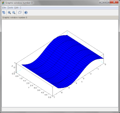
The grid is generated by specifying two vectors giving the coordinates along the x- and y-axes. The grid is obtained by computing the coordinates of all intersection points. A third vector specifies the z coordinates of the intersection points of the grid. Thus, if x is a vector of size mx1, and y is a vector of size 1xn, then z is a matrix of size mxn. Study the following example:

-->x = [0:%pi/16:2*%pi]'; // Note the transpose. Size is 33x1
-->y = [0:5]; // Size 1x6
-->z = sin(x) * ones(y); // ones(y) has same size as y and all elements are 1
-->size(x), size(y), size(z)
 ans  =
    33.  1.
 ans  =
    1.   6.
 ans  =
    33.   6.
-->plot3d(x, y, z)

Function plot3d1() is similar to function plot3d(), except that it produces a colour level plot of the surface, using the same colour for points with same height (or for points lying within a certain range of height).

3D Graphs using Facets

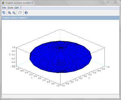
Function plot3d2() generates surfaces using facets rather than grids. Here, the arguments to the function, namely, x, y and z are two dimensional matrices. The surface is composed of four sided polygons, with the x coordinate of the polygon stored in x(i, j), x(i+1, j), x(i, j+1) and x(i+1, j+1). Similarly, the y and z coordinates of the polygons are stored in the y and z matrices.

In the following example, we will use the function linspace(s1, s2, n) to generate n equally spaced values with s1 as the start value and s2 as the end value. Thus linspace(0, 10, 11) is equivalent to the range 0:10. Similarly, linspace(0, 10, 21) is the same as the range 0:0.5:10.

-->u = linspace(-%pi/2, %pi/2, 40); size(u)
 ans  =
     1.  40.
-->v = linspace(0, 2*%pi, 20); size(v)
 ans  =
     1.  20.
-->x = cos(u)' * cos(v); size(x) // cos(u)' is of size 40x1, cos(v) is 1x20
 ans  =
     40.  20.
-->y = cos(u)' * sin(u);
-->z = sin(u)' * ones(v);
-->plot3d2(x, y, z)

Plottimg Multiples Graphs using subplot()

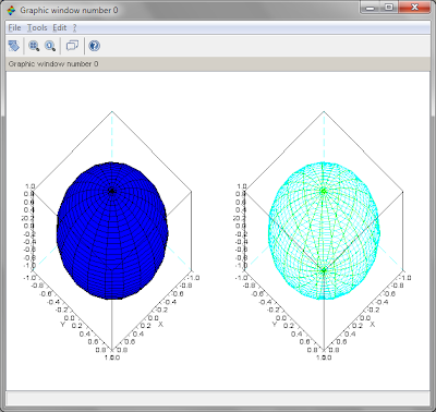
Function subplot() is used to plot multiple graphs within one graphics window. Thesubplot() command must immediately precede a plotting command in order to produce a sub-plot. The subplot() function logically divides the graphic window into an array of rows and columns, and chooses one of the cells as the output of the subsequent plotting command. For example, subplot(235) divides the window into two rows and 3 columns (that is 6 cells in all). Cells are counted in sequence starting from top left proceeding to the right first and then down. Therefore cell 5 in the above command implies that the output of the next plotting command will be sent to the cell on row 2, column 2.

-->clf(); subplot(121); plot3d2(x, y, z); subplot(122); plot3d3(x, y, z)

Exporting Graphs

Graphs can be exported to one of the following formats: PNG, PPM, EMF, EPS, FIG, PDF and SVG. To export the contents of the graphics window, go to the main menu of the graphics window and choose File -> Export to (Ctrl+E). This opens a dialog box where you can choose the filename for the image file and its file type. The image cn then be imported into a document.